Event Study (Dynamic DiD) with pymc models#
This notebook demonstrates how to use CausalPy’s EventStudy class to estimate dynamic treatment effects over event time. This is also known as a “dynamic difference in differences” analysis. The event study is a powerful tool for:
Examining pre-treatment trends (placebo checks for parallel trends assumption)
Estimating how treatment effects evolve over time after treatment
Visualizing the full time path of causal effects
Background: What is an Event Study?#
An event study analyzes panel data where some units receive treatment at a specific time. Unlike standard difference-in-differences which estimates a single average treatment effect, event studies estimate separate coefficients for each time period relative to treatment [Roth et al., 2023, Baker et al., 2025].
The key concept is event time (or relative time):
where \(t\) is the calendar time and \(G_i\) is the treatment time for unit \(i\).
The model estimates [Sun and Abraham, 2021]:
where:
\(\alpha_i\) are unit fixed effects
\(\lambda_t\) are time fixed effects
\(\beta_k\) are the dynamic treatment effects at event time \(k\)
\(k_0\) is the reference (omitted) period, typically \(k=-1\)
\(\mathbf{1}\{E_{it} = k\}\) is the indicator function: it equals 1 when the condition inside the braces is true (i.e., when observation \(it\) is at event time \(k\)), and 0 otherwise
Understanding the Indicator Function as Dummy Variables#
The indicator function notation \(\mathbf{1}\{E_{it} = k\}\) is mathematically equivalent to creating dummy (binary) variables. For each event time \(k\) in the event window:
Create a dummy variable \(D_k\) that equals 1 for treated units at event time \(k\), and 0 otherwise
Omit one event time (the reference period, typically \(k=-1\)) to avoid perfect multicollinearity
This means the summation \(\sum_{k \neq k_0} \beta_k \cdot \mathbf{1}\{E_{it} = k\}\) is equivalent to including dummy variables \(D_{-5}, D_{-4}, ..., D_0, D_1, ...\) (excluding \(D_{-1}\)) in your regression.
Key insight: The estimated regression coefficient \(\beta_k\) for each dummy variable represents the Average Treatment Effect on the Treated (ATT) at event time \(k\), measured relative to the reference period. Since the reference period (\(k=-1\)) is omitted, its coefficient is implicitly zero, and all other coefficients show the difference from that baseline.
Interpretation:
\(\beta_k\) for \(k < 0\) (pre-treatment): Should be near zero if parallel trends hold
\(\beta_k\) for \(k \geq 0\) (post-treatment): Measure the causal effect at each period after treatment
Warning
This implementation uses a standard two-way fixed effects (TWFE) estimator, which requires simultaneous treatment timing - all treated units must receive treatment at the same time. Staggered adoption designs (where different units are treated at different times) can produce biased estimates when treatment effects vary across cohorts [Goodman-Bacon, 2021, Sun and Abraham, 2021, Callaway and Sant'Anna, 2021]. For comprehensive guidance on modern DiD methods that address these issues, see Baker et al. [2025] and Roth et al. [2023].
import textwrap

import arviz as az
import matplotlib.pyplot as plt
import seaborn as sns

import causalpy as cp
from causalpy.data.simulate_data import generate_event_study_data
%load_ext autoreload
%autoreload 2
%config InlineBackend.figure_format = 'retina'
seed = 42
# Set arviz style to override seaborn's default
az.style.use("arviz-darkgrid")
Generate Simulated Data#
We’ll create synthetic panel data with:
30 units (half treated, half control)
20 time periods
Treatment occurring at time 10
Known treatment effects: zero pre-treatment, gradually increasing post-treatment
# Define known treatment effects for simulation
# Pre-treatment: no effect (parallel trends)
# Post-treatment: effect increases over time
true_effects = {
    -5: 0.0,
    -4: 0.0,
    -3: 0.0,
    -2: 0.0,
    -1: 0.0,  # Pre-treatment
    0: 0.5,
    1: 0.7,
    2: 0.9,
    3: 1.0,
    4: 1.0,
    5: 1.0,  # Post-treatment
}

df = generate_event_study_data(
    n_units=30,
    n_time=20,
    treatment_time=10,
    treated_fraction=0.5,
    event_window=(-5, 5),
    treatment_effects=true_effects,
    unit_fe_sigma=1.0,
    time_fe_sigma=0.3,
    noise_sigma=0.2,
    seed=seed,
)

print(f"Data shape: {df.shape}")
df.head(10)
Data shape: (600, 5)
| unit | time | y | treat_time | treated | |
|---|---|---|---|---|---|
| 0 | 0 | 0 | 0.381019 | 10.0 | 1 |
| 1 | 0 | 1 | 0.975381 | 10.0 | 1 |
| 2 | 0 | 2 | 0.357281 | 10.0 | 1 |
| 3 | 0 | 3 | 0.301736 | 10.0 | 1 |
| 4 | 0 | 4 | 0.949678 | 10.0 | 1 |
| 5 | 0 | 5 | 0.316717 | 10.0 | 1 |
| 6 | 0 | 6 | 0.391530 | 10.0 | 1 |
| 7 | 0 | 7 | -0.153029 | 10.0 | 1 |
| 8 | 0 | 8 | 0.164511 | 10.0 | 1 |
| 9 | 0 | 9 | 0.750882 | 10.0 | 1 |
Let’s visualize the data to understand its structure:
Show code cell source
fig, ax = plt.subplots(figsize=(8, 5))
sns.lineplot(
    data=df,
    x="time",
    y="y",
    hue="treated",
    units="unit",
    estimator=None,
    alpha=0.5,
    ax=ax,
)
ax.axvline(x=10, color="red", linestyle="--", linewidth=2, label="Treatment time")
ax.set(
    xlabel="Time", ylabel="Outcome (y)", title="Panel Data: Treated vs Control Units"
)
ax.legend(loc="upper left")
plt.show()

Event Study Analysis #1#
Now we use CausalPy’s EventStudy class to estimate the dynamic treatment effects.
The formula parameter uses patsy syntax to specify the model structure:
y ~ C(unit) + C(time)specifies the outcome variableywith unit fixed effects (\(\alpha_i\)) and time fixed effects (\(\lambda_t\))C(column)indicates a categorical variable that should be converted to dummy variables
What about the \(\beta_k\) coefficients? These are the event-time dummies - the key parameters we want to estimate. They capture the treatment effect at each period relative to treatment (i.e., at each event time \(k\)). The class automatically constructs these based on:
The
event_windowparameter (e.g.,(-5, 5)means \(k \in \{-5, -4, ..., 0, ..., 5\}\))The
reference_event_timeparameter (e.g.,-1is omitted as the baseline)
So the formula specifies the “structural” part of the model (\(\alpha_i + \lambda_t\)), while the event-time dummies (\(\sum_{k \neq k_0} \beta_k \cdot \mathbf{1}\{E_{it} = k\}\)) are added automatically.
Note
The random_seed keyword argument for the PyMC sampler is not necessary. We use it here so that the results are reproducible.
result = cp.EventStudy(
    df,
    formula="y ~ C(unit) + C(time)",  # Outcome with unit and time fixed effects
    unit_col="unit",
    time_col="time",
    treat_time_col="treat_time",
    event_window=(-5, 5),
    reference_event_time=-1,  # One period before treatment as reference
    model=cp.pymc_models.LinearRegression(sample_kwargs={"random_seed": seed}),
)
Show code cell output
Initializing NUTS using jitter+adapt_diag...
Multiprocess sampling (4 chains in 4 jobs)
NUTS: [beta, y_hat_sigma]
Sampling 4 chains for 1_000 tune and 1_000 draw iterations (4_000 + 4_000 draws total) took 2 seconds.
The rhat statistic is larger than 1.01 for some parameters. This indicates problems during sampling. See https://arxiv.org/abs/1903.08008 for details
The effective sample size per chain is smaller than 100 for some parameters.  A higher number is needed for reliable rhat and ess computation. See https://arxiv.org/abs/1903.08008 for details
Sampling: [beta, y_hat, y_hat_sigma]
Sampling: [y_hat]
Visualize the Results#
The event study plot shows the estimated treatment effects (\(\beta_k\)) at each event time, with credible intervals. This is the key diagnostic plot for event studies.
fig, ax = result.plot(figsize=(8, 5))
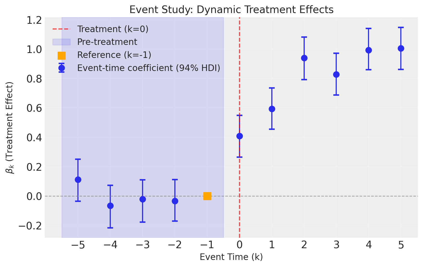
Interpreting the Plot:
Pre-treatment periods (\(k < 0\), blue shaded): The coefficients should be close to zero. This is a key test of the parallel trends assumption. If we see significant pre-trends, our causal estimates may be biased.
Reference period (\(k = -1\), orange square): This is fixed at zero by construction. All other coefficients are interpreted relative to this period.
Post-treatment periods (\(k \geq 0\)): These show how the treatment effect evolves over time. In our simulated data, we see the effect starts at about 0.5 and increases to around 1.0.
Credible intervals: The error bars show 94% highest density intervals. When these don’t include zero for post-treatment periods, we have strong evidence of a treatment effect.
Tip
The plot can be customized with optional parameters:
figsize=(width, height)to change the figure sizehdi_prob=0.89to change the credible interval (e.g., 89% instead of 94%)
Example: result.plot(figsize=(12, 8), hdi_prob=0.89)
Summary Statistics#
result.summary()
==================================Event Study===================================
Formula: y ~ C(unit) + C(time)
Event window: (-5, 5)
Reference event time: -1

Event-time coefficients (beta_k):
------------------------------------------------------------
  Event Time       Mean         SD     HDI 3%    HDI 97%
------------------------------------------------------------
          -5       0.11      0.077     -0.035       0.25
          -4     -0.065      0.077      -0.22      0.073
          -3     -0.021      0.078      -0.18       0.11
          -2     -0.032      0.075      -0.17       0.11
          -1    0 (ref)          -          -          -
           0       0.41      0.076       0.26       0.55
           1       0.59      0.075       0.45       0.74
           2       0.94      0.078       0.79        1.1
           3       0.83      0.075       0.69       0.97
           4       0.99      0.075       0.86        1.1
           5          1      0.076       0.86        1.1
------------------------------------------------------------
Model coefficients:
    Intercept      0.3, 94% HDI [0.19, 0.4]
    C(unit)[T.1]   -0.64, 94% HDI [-0.76, -0.52]
    C(unit)[T.2]   0.12, 94% HDI [-0.0064, 0.24]
    C(unit)[T.3]   1, 94% HDI [0.91, 1.2]
    C(unit)[T.4]   -0.78, 94% HDI [-0.9, -0.66]
    C(unit)[T.5]   -0.7, 94% HDI [-0.82, -0.58]
    C(unit)[T.6]   1.1, 94% HDI [0.96, 1.2]
    C(unit)[T.7]   0.3, 94% HDI [0.18, 0.42]
    C(unit)[T.8]   -0.97, 94% HDI [-1.1, -0.85]
    C(unit)[T.9]   0.032, 94% HDI [-0.085, 0.15]
    C(unit)[T.10]  -1, 94% HDI [-1.1, -0.9]
    C(unit)[T.11]  -0.96, 94% HDI [-1.1, -0.84]
    C(unit)[T.12]  -0.24, 94% HDI [-0.36, -0.12]
    C(unit)[T.13]  -2.4, 94% HDI [-2.5, -2.2]
    C(unit)[T.14]  -2.3, 94% HDI [-2.4, -2.2]
    C(unit)[T.15]  -1.1, 94% HDI [-1.2, -0.94]
    C(unit)[T.16]  -1.5, 94% HDI [-1.6, -1.4]
    C(unit)[T.17]  -0.22, 94% HDI [-0.35, -0.097]
    C(unit)[T.18]  -1.4, 94% HDI [-1.5, -1.2]
    C(unit)[T.19]  -2, 94% HDI [-2.1, -1.9]
    C(unit)[T.20]  0.91, 94% HDI [0.79, 1]
    C(unit)[T.21]  -0.75, 94% HDI [-0.87, -0.63]
    C(unit)[T.22]  -0.48, 94% HDI [-0.6, -0.36]
    C(unit)[T.23]  -2, 94% HDI [-2.1, -1.9]
    C(unit)[T.24]  -1.1, 94% HDI [-1.2, -1]
    C(unit)[T.25]  -0.43, 94% HDI [-0.55, -0.31]
    C(unit)[T.26]  -1.6, 94% HDI [-1.8, -1.5]
    C(unit)[T.27]  -0.14, 94% HDI [-0.26, -0.011]
    C(unit)[T.28]  -1, 94% HDI [-1.2, -0.92]
    C(unit)[T.29]  -0.9, 94% HDI [-1, -0.78]
    C(time)[T.1]   0.8, 94% HDI [0.7, 0.89]
    C(time)[T.2]   0.22, 94% HDI [0.12, 0.31]
    C(time)[T.3]   -0.043, 94% HDI [-0.14, 0.05]
    C(time)[T.4]   0.53, 94% HDI [0.44, 0.62]
    C(time)[T.5]   -0.23, 94% HDI [-0.35, -0.11]
    C(time)[T.6]   0.32, 94% HDI [0.2, 0.44]
    C(time)[T.7]   -0.38, 94% HDI [-0.51, -0.27]
    C(time)[T.8]   -0.14, 94% HDI [-0.25, -0.018]
    C(time)[T.9]   0.28, 94% HDI [0.18, 0.37]
    C(time)[T.10]  0.49, 94% HDI [0.37, 0.6]
    C(time)[T.11]  0.35, 94% HDI [0.24, 0.47]
    C(time)[T.12]  0.14, 94% HDI [0.015, 0.26]
    C(time)[T.13]  0.24, 94% HDI [0.11, 0.35]
    C(time)[T.14]  -0.25, 94% HDI [-0.37, -0.13]
    C(time)[T.15]  -0.0026, 94% HDI [-0.13, 0.11]
    C(time)[T.16]  0.044, 94% HDI [-0.05, 0.14]
    C(time)[T.17]  0.5, 94% HDI [0.4, 0.59]
    C(time)[T.18]  0.34, 94% HDI [0.24, 0.43]
    C(time)[T.19]  -0.32, 94% HDI [-0.42, -0.23]
    event_time_-5  0.11, 94% HDI [-0.033, 0.26]
    event_time_-4  -0.065, 94% HDI [-0.21, 0.079]
    event_time_-3  -0.021, 94% HDI [-0.17, 0.12]
    event_time_-2  -0.032, 94% HDI [-0.17, 0.11]
    event_time_0   0.41, 94% HDI [0.27, 0.55]
    event_time_1   0.59, 94% HDI [0.45, 0.73]
    event_time_2   0.94, 94% HDI [0.8, 1.1]
    event_time_3   0.83, 94% HDI [0.69, 0.97]
    event_time_4   0.99, 94% HDI [0.85, 1.1]
    event_time_5   1, 94% HDI [0.86, 1.2]
    y_hat_sigma    0.2, 94% HDI [0.19, 0.21]
Effect Summary#
The effect_summary() method provides a decision-ready summary with both a table and prose description. It automatically includes a parallel trends check that examines whether pre-treatment coefficients are consistent with the identifying assumption:
effect = result.effect_summary()
wrapped = textwrap.fill(effect.text, width=75)
print(wrapped)
Event study analysis with 11 time periods (k=-5 to k=5), reference period
k=-1. Pre-treatment coefficients (k<0) are consistent with the parallel
trends assumption (all 95% HDIs include zero). Post-treatment effects (k≥0)
show treatment impact ranging from 0.41 to 1.01.
effect.table
| event_time | mean | std | hdi_3% | hdi_98% | is_reference | |
|---|---|---|---|---|---|---|
| 0 | -5 | 0.113427 | 0.076994 | -0.035227 | 0.263490 | False |
| 1 | -4 | -0.064592 | 0.076905 | -0.223268 | 0.077255 | False |
| 2 | -3 | -0.021091 | 0.077551 | -0.176982 | 0.122292 | False |
| 3 | -2 | -0.032195 | 0.074954 | -0.180698 | 0.112547 | False |
| 4 | -1 | 0.000000 | 0.000000 | 0.000000 | 0.000000 | True |
| 5 | 0 | 0.409094 | 0.075700 | 0.264175 | 0.559484 | False |
| 6 | 1 | 0.593974 | 0.075284 | 0.442126 | 0.735045 | False |
| 7 | 2 | 0.940384 | 0.077661 | 0.791473 | 1.092842 | False |
| 8 | 3 | 0.827706 | 0.075419 | 0.679464 | 0.972220 | False |
| 9 | 4 | 0.992739 | 0.075394 | 0.848039 | 1.139731 | False |
| 10 | 5 | 1.006455 | 0.075720 | 0.861012 | 1.158448 | False |
Tip
You can disable the parallel trends check in the prose by passing include_pretrend_check=False:
result.effect_summary(include_pretrend_check=False)
We can also get the event-time coefficients as a DataFrame directly like this:
summary_df = result.get_event_time_summary()
summary_df
| event_time | mean | std | hdi_3% | hdi_97% | is_reference | |
|---|---|---|---|---|---|---|
| 0 | -5 | 0.113427 | 0.076994 | -0.035227 | 0.251823 | False |
| 1 | -4 | -0.064592 | 0.076905 | -0.215547 | 0.073316 | False |
| 2 | -3 | -0.021091 | 0.077551 | -0.177766 | 0.111183 | False |
| 3 | -2 | -0.032195 | 0.074954 | -0.169954 | 0.112547 | False |
| 4 | -1 | 0.000000 | 0.000000 | 0.000000 | 0.000000 | True |
| 5 | 0 | 0.409094 | 0.075700 | 0.264636 | 0.548505 | False |
| 6 | 1 | 0.593974 | 0.075284 | 0.454389 | 0.735734 | False |
| 7 | 2 | 0.940384 | 0.077661 | 0.792238 | 1.081568 | False |
| 8 | 3 | 0.827706 | 0.075419 | 0.688432 | 0.971350 | False |
| 9 | 4 | 0.992739 | 0.075394 | 0.860349 | 1.140122 | False |
| 10 | 5 | 1.006455 | 0.075720 | 0.862488 | 1.148255 | False |
Compare Estimated vs True Effects#
Since we simulated the data with known treatment effects, we can compare our estimates to the true values. We would not be able to do this with real-world data where the ground truth is unknown.
Show code cell source
fig, ax = plt.subplots(figsize=(8, 5))

# Plot estimated effects
event_times = summary_df["event_time"].values
estimated_means = summary_df["mean"].values
lower = summary_df["hdi_3%"].values
upper = summary_df["hdi_97%"].values

ax.errorbar(
    event_times,
    estimated_means,
    yerr=[estimated_means - lower, upper - estimated_means],
    fmt="o",
    capsize=4,
    capthick=2,
    markersize=8,
    color="C0",
    label="Estimated (with 94% HDI)",
)

# Plot true effects (relative to k=-1 reference)
# Since k=-1 is our reference, we need to subtract true_effects[-1] from all
true_effects_relative = {k: v - true_effects[-1] for k, v in true_effects.items()}
true_k = list(true_effects_relative.keys())
true_beta = list(true_effects_relative.values())
ax.scatter(
    true_k, true_beta, marker="x", s=100, color="red", zorder=5, label="True effect"
)

ax.axhline(y=0, color="gray", linestyle="--", alpha=0.7)
ax.axvline(x=0, color="gray", linestyle=":", alpha=0.7)
ax.set_xlabel("Event Time (k)")
ax.set_ylabel(r"$\beta_k$ (Treatment Effect)")
ax.set_title("Estimated vs True Treatment Effects")
ax.legend()
ax.grid(True, alpha=0.3)
plt.show()
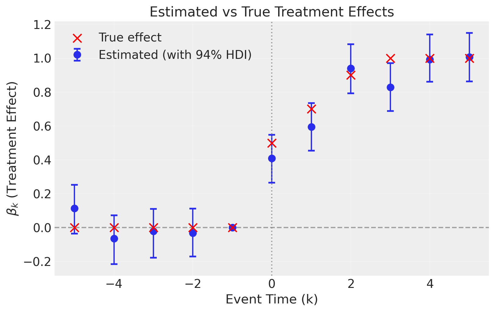
The estimated effects closely track the true effects, demonstrating that the event study correctly recovers the dynamic treatment effects.
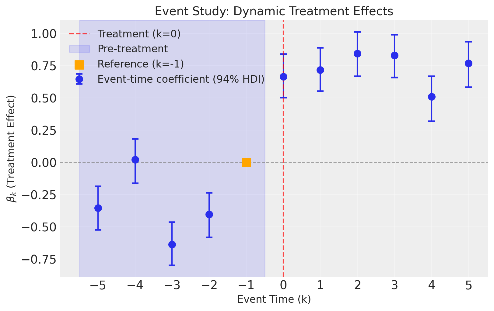
Event Study Analysis #2#
Now we’ll run an event study analysis but without a time fixed effect.
result2 = cp.EventStudy(
    df,
    formula="y ~ C(unit)",  # Outcome with unit fixed effects, no time fixed effects
    unit_col="unit",
    time_col="time",
    treat_time_col="treat_time",
    event_window=(-5, 5),
    reference_event_time=-1,  # One period before treatment as reference
    model=cp.pymc_models.LinearRegression(sample_kwargs={"random_seed": seed}),
)
Initializing NUTS using jitter+adapt_diag...
Multiprocess sampling (4 chains in 4 jobs)
NUTS: [beta, y_hat_sigma]
Sampling 4 chains for 1_000 tune and 1_000 draw iterations (4_000 + 4_000 draws total) took 2 seconds.
The effective sample size per chain is smaller than 100 for some parameters.  A higher number is needed for reliable rhat and ess computation. See https://arxiv.org/abs/1903.08008 for details
Sampling: [beta, y_hat, y_hat_sigma]
Sampling: [y_hat]
fig, ax = result2.plot(figsize=(8, 5))
summary_df = result2.get_event_time_summary()
summary_df
| event_time | mean | std | hdi_3% | hdi_97% | is_reference | |
|---|---|---|---|---|---|---|
| 0 | -5 | -0.353136 | 0.090493 | -0.522287 | -0.186003 | False |
| 1 | -4 | 0.021606 | 0.091856 | -0.161145 | 0.181621 | False |
| 2 | -3 | -0.635135 | 0.089622 | -0.797790 | -0.462520 | False |
| 3 | -2 | -0.403374 | 0.092969 | -0.582083 | -0.234025 | False |
| 4 | -1 | 0.000000 | 0.000000 | 0.000000 | 0.000000 | True |
| 5 | 0 | 0.666587 | 0.091566 | 0.503798 | 0.839579 | False |
| 6 | 1 | 0.716158 | 0.091080 | 0.552381 | 0.888947 | False |
| 7 | 2 | 0.844532 | 0.093367 | 0.667764 | 1.012533 | False |
| 8 | 3 | 0.829304 | 0.089390 | 0.659251 | 0.989613 | False |
| 9 | 4 | 0.508772 | 0.091841 | 0.319907 | 0.667985 | False |
| 10 | 5 | 0.768295 | 0.094161 | 0.582870 | 0.937573 | False |
We can see that not including time fixed effects means that we are unable to account for time-based shocks that affect all units identically. The consequence of this is that our causal estimates (the dynamic treatment effects) are now biased. This is most noticeable with the pre-intervention placebo checks, where we see meaningful deviations from zero effect before the intervention.
Event Study Analysis #3: With Time-Varying Predictors#
In real-world applications, outcomes often depend on time-varying covariates beyond the treatment itself. For example, sales might be affected by temperature, economic indicators, or seasonal factors.
The generate_event_study_data function supports generating time-varying predictors via AR(1) processes. These predictors:
Vary smoothly over time (controlled by the
ar_phipersistence parameter)Are the same for all units at a given time period
Contribute to the outcome through user-specified coefficients
The data generating process becomes:
where \(X_{jt}\) are the time-varying predictors and \(\gamma_j\) are their true coefficients.
# Generate data with two time-varying predictors
# - temperature: positive effect on outcome (coefficient = 0.3)
# - humidity: negative effect on outcome (coefficient = -0.2)
df_predictors = generate_event_study_data(
    n_units=30,
    n_time=20,
    treatment_time=10,
    treated_fraction=0.5,
    event_window=(-5, 5),
    treatment_effects=true_effects,
    unit_fe_sigma=1.0,
    time_fe_sigma=0.3,
    noise_sigma=0.2,
    predictor_effects={"temperature": 0.3, "humidity": -0.2},
    ar_phi=0.9,  # High persistence for smooth variation
    ar_scale=1.0,
    seed=seed,
)

print(f"Data shape: {df_predictors.shape}")
print(f"Columns: {df_predictors.columns.tolist()}")
df_predictors.head(10)
Data shape: (600, 7)
Columns: ['unit', 'time', 'y', 'treat_time', 'treated', 'temperature', 'humidity']
| unit | time | y | treat_time | treated | temperature | humidity | |
|---|---|---|---|---|---|---|---|
| 0 | 0 | 0 | 0.210250 | 10.0 | 1 | 0.000000 | 0.000000 |
| 1 | 0 | 1 | 1.381300 | 10.0 | 1 | 0.324084 | -0.645120 |
| 2 | 0 | 2 | 0.527901 | 10.0 | 1 | -0.093407 | -0.219212 |
| 3 | 0 | 3 | -0.123316 | 10.0 | 1 | -0.760988 | 1.340746 |
| 4 | 0 | 4 | 0.346934 | 10.0 | 1 | -0.073213 | 1.170845 |
| 5 | 0 | 5 | -0.169220 | 10.0 | 1 | 0.965108 | 2.618404 |
| 6 | 0 | 6 | 1.073551 | 10.0 | 1 | 1.799877 | -0.263181 |
| 7 | 0 | 7 | -0.266696 | 10.0 | 1 | 0.780672 | 0.585039 |
| 8 | 0 | 8 | 0.152784 | 10.0 | 1 | 0.393392 | 0.613582 |
| 9 | 0 | 9 | 0.762935 | 10.0 | 1 | 0.685317 | 0.253217 |
Show code cell source
# Visualize the time-varying predictors
# Since predictors are the same for all units at each time, we just need one unit's data
predictor_data = df_predictors[df_predictors["unit"] == 0][
    ["time", "temperature", "humidity"]
]

fig, axes = plt.subplots(1, 2, figsize=(12, 4))

axes[0].plot(predictor_data["time"], predictor_data["temperature"], marker="o")
axes[0].axvline(x=10, color="red", linestyle="--", alpha=0.7, label="Treatment time")
axes[0].set(xlabel="Time", ylabel="Temperature", title="Temperature (AR(1) process)")
axes[0].legend()

axes[1].plot(predictor_data["time"], predictor_data["humidity"], marker="o", color="C1")
axes[1].axvline(x=10, color="red", linestyle="--", alpha=0.7, label="Treatment time")
axes[1].set(xlabel="Time", ylabel="Humidity", title="Humidity (AR(1) process)")
axes[1].legend()

plt.suptitle("Time-Varying Predictors Generated via AR(1) Processes", y=1.02)
plt.tight_layout()
plt.show()
/var/folders/r0/nf1kgxsx6zx3rw16xc3wnnzr0000gn/T/ipykernel_63830/1024805842.py:20: UserWarning: The figure layout has changed to tight
  plt.tight_layout()

Show code cell source
fig, ax = plt.subplots(figsize=(8, 5))
sns.lineplot(
    data=df_predictors,
    x="time",
    y="y",
    hue="treated",
    units="unit",
    estimator=None,
    alpha=0.5,
    ax=ax,
)
ax.axvline(x=10, color="red", linestyle="--", linewidth=2, label="Treatment time")
ax.set(
    xlabel="Time", ylabel="Outcome (y)", title="Panel Data: Treated vs Control Units"
)
ax.legend(loc="upper left")
plt.show()

Now we run the event study, including the predictors in the formula. This allows the model to control for the time-varying confounders:
result3 = cp.EventStudy(
    df_predictors,
    formula="y ~ temperature + humidity + C(unit) + C(time)",
    unit_col="unit",
    time_col="time",
    treat_time_col="treat_time",
    event_window=(-5, 5),
    reference_event_time=-1,
    model=cp.pymc_models.LinearRegression(sample_kwargs={"random_seed": seed}),
)
Show code cell output
Initializing NUTS using jitter+adapt_diag...
Multiprocess sampling (4 chains in 4 jobs)
NUTS: [beta, y_hat_sigma]
Sampling 4 chains for 1_000 tune and 1_000 draw iterations (4_000 + 4_000 draws total) took 72 seconds.
Chain 0 reached the maximum tree depth. Increase `max_treedepth`, increase `target_accept` or reparameterize.
Chain 1 reached the maximum tree depth. Increase `max_treedepth`, increase `target_accept` or reparameterize.
Chain 2 reached the maximum tree depth. Increase `max_treedepth`, increase `target_accept` or reparameterize.
Chain 3 reached the maximum tree depth. Increase `max_treedepth`, increase `target_accept` or reparameterize.
The rhat statistic is larger than 1.01 for some parameters. This indicates problems during sampling. See https://arxiv.org/abs/1903.08008 for details
The effective sample size per chain is smaller than 100 for some parameters.  A higher number is needed for reliable rhat and ess computation. See https://arxiv.org/abs/1903.08008 for details
Sampling: [beta, y_hat, y_hat_sigma]
Sampling: [y_hat]
fig, ax = result3.plot(figsize=(8, 5))
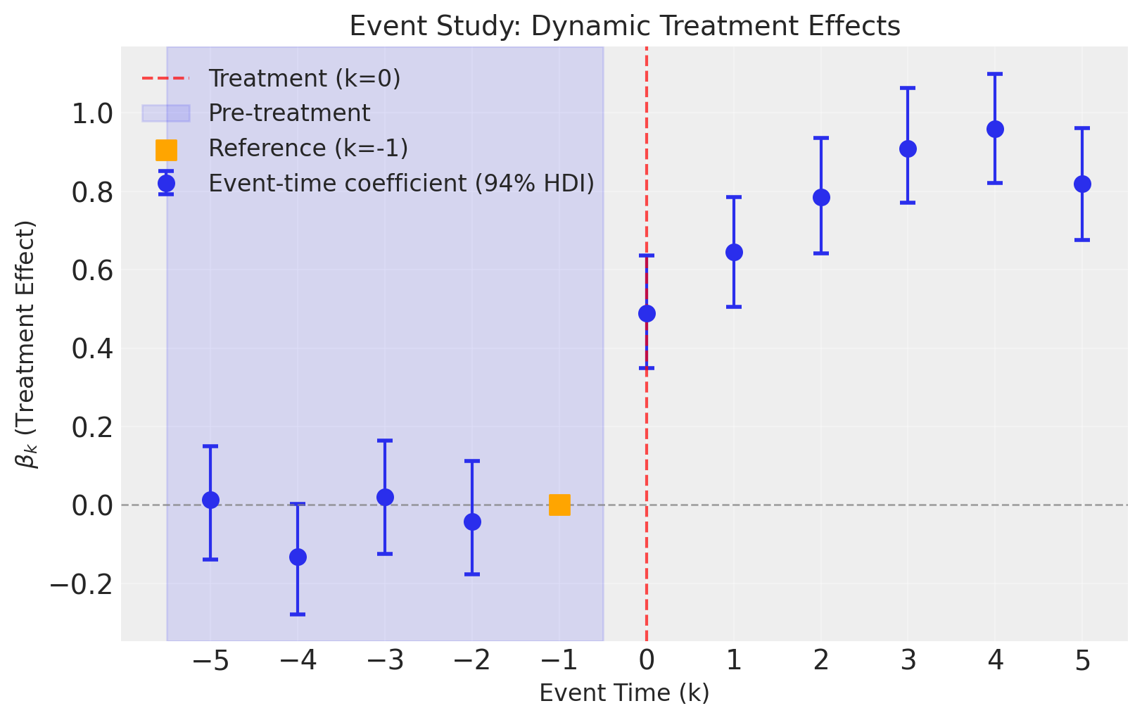
The event study correctly recovers the dynamic treatment effects even in the presence of time-varying predictors.
Key Takeaways#
Event studies provide richer information than standard DiD by estimating treatment effects at each event time [Roth et al., 2023, Baker et al., 2025].
Pre-trend analysis is crucial: the
effect_summary()method automatically checks whether pre-treatment coefficients (\(k < 0\)) are consistent with the parallel trends assumption.Dynamic effects can reveal how treatment impacts evolve over time—whether effects are immediate, gradual, or temporary.
The reference period (\(k_0\), typically -1) is normalized to zero. All coefficients are interpreted relative to this period.
Bayesian estimation provides full posterior distributions for each coefficient, enabling probabilistic statements about effect sizes.
Time-varying predictors can be included in the model formula to control for confounders. The
generate_event_study_datafunction supports generating AR(1) predictors with user-specified coefficients for realistic simulations.Implementation considerations: This notebook demonstrates event studies with simultaneous treatment timing. For staggered adoption designs, specialized estimators are required to avoid bias from treatment effect heterogeneity [Goodman-Bacon, 2021, Sun and Abraham, 2021, Callaway and Sant'Anna, 2021]. See Baker et al. [2025] for a comprehensive practitioner’s guide to DiD designs.
References#
Andrew Goodman-Bacon. Difference-in-differences with variation in treatment timing. Journal of Econometrics, 225(2):254–277, 2021.
Jonathan Roth, Pedro HC Sant'Anna, Alyssa Bilinski, and John Poe. What's trending in difference-in-differences? a synthesis of the recent econometrics literature. Journal of Econometrics, 235(2):2218–2244, 2023.
Andrew Baker, Brantly Callaway, Scott Cunningham, Andrew Goodman-Bacon, and Pedro HC Sant'Anna. Difference-in-differences designs: a practitioner's guide. arXiv preprint arXiv:2503.13323, 2025. URL: https://arxiv.org/abs/2503.13323.